Check out the basic information of Loop the Loop here.
Visually, Loop the Loop appears to be a simple paper-and-pencil game but once one is introduced to the gameplay, its complexity evolves quite quickly. The game consists of two players, both of which agree on a number of small loops to draw within one large loop, which could be considered the game board. The arbitrarily declared first player must find a group of four or more loops inside a larger loop and draw a loop around three or more of these loops but not all of them. For clarity, the group of internal loops will be called “micro-loops” and their mutually external loop will be called the “macro-loop”. One of the key rules of the game states that micro-loops and their respective macro-loop are collectively considered one micro-loop within the macro-loop’s respective macro-loop. The game is sequential and therefore the two players alternate turns. The game continues until one of the players makes the last legal move and is declared the winner.
The freedom that Loop the Loop provides to its players enables the existence of incredibly intricate game state paths. In order to better comprehend the game, one needs to map out some of the possible gameplays and attempt to perceive some sort of pattern. This analysis begins with a game board in which the initial amount of micro-loops within the macro-loop is four since four is the minimum number of pieces for a playable game of Loop the Loop. The first player would enact the only possible move, circling three of the micro-loops and converting them into one micro-loop within the whole game board. No more moves are possible since there are only two micro-loops within the game board, the largest loop, and there are less than four micro-loops within the only macro-loop in the board. Hence, for a game board of initially four micro-loops, the first player is the automatic winner. Clearly, Loop the Loop can be identified as a normal game since the first player performed the last possible move and won.
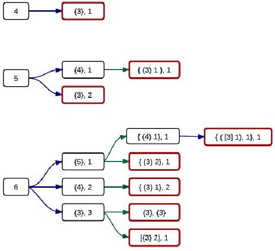
Figure 1 (click to view enlarged)
The next game board is one initially beginning with five micro-loops. Now the first player has two moves to choose from: either circling three or four of the micro-loops. However, it would be in the first player’s interest to circle only three of them, such that there are no more possible moves and the second player loses. If the first player were to circle four of the micro-loops, then the second player could win the game by circling three of those micro-loops within the new macro-loop, with no more possible moves remaining. As one continues to add one micro-loop to the initial game board, it seems that a pattern exists such that the number of possible moves the first player can makes increases by one. Thus, the number of possible first moves of the game is the difference between the number of total initial micro-loops and three, n – 3. Another noted pattern when adding one micro-loop to the initial game board is that the degree of maximum possible moves of the game increases by one. For example, with a game board of six, it takes a maximum of three moves for the game to end. Up to four moves can be played sequentially on a game board of seven micro-loops. A game with a board of eight micro-loops ends in a maximum of five moves.
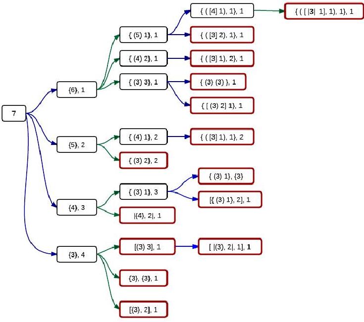
Figure 2 (click to view enlarged)
Hence, the degree of maximum possible moves also has a relationship with the initial number of micro-loops such that the difference between the total initial micro-loops and three is equal to the degree of maximum moves, n – 3. These patterns can be clearly demonstrated in a set of tree graphs, as shown below in Figures 1, 2, and 3, where blue arrows represent all the possible first player moves, green arrows represent all the possible second player moves, the boxes represent the entire game board, a set of identical brackets represents a macro-loop, a set of identical brackets within a set of identical brackets represents a macro-loop within a larger macro-loop, the numbers represent the initial micro-loops of the game board, and the red boxes represent terminal positions. Note that the tree graphs only represent the game boards that hold the initial number of micro-loops four through eight. This is due to the continually growing intricacy of the game board past eight initial micro-loops.
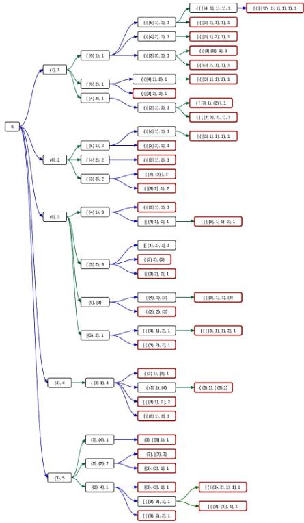
Figure 3 (click to view enlarged)
By now, other aspects of Loop the Loop can be classified. The game is determinate since there are clear paths of sequential game states that depend only on the moves a player can make, as demonstrated by the tree graphs, not on random chance. The game is zero-sum since there is a winner and a loser for each time the game is played; one of the player's gains is equal to the other player's losses. The game is also asymmetric since the pay-off of the game depends on which player employs a specific strategy. For example, once the first player creates the first loop, the different loops that the second player can make changes. Loop the Loop is a game of perfect information as there are no unknown variables and both players can determine all the possible game states, with time of course. Furthermore, the game is unfair. There are clear game play paths that one of both players, depending on the number of initial micro-loops, can take such that that player can play optimally and win. For example, for a game board of initially six loops, the second player will always win if the individual plays optimally. For all the other game boards demonstrated in the tree graphs, the first player, if playing optimally, always wins. Due to the continually developing intricacy of the game, as one increases the number of initial micro-loops, and the continual branching out of the game's tree graphs, it is hypothetical that there will always be a path such that the first player will always win if playing optimally no matter what the second player does. Finally, Loop the Loop can be generally considered as an impartial, combinatorial game. Thomas Ferguson characterizes an impartial combinatorial game as a game with: two players, a set of possible positions of the game, specific rules for both players and positions such that both players have the same options of moving from each position, alternating moves between players, terminal positions at which the game ends, and the condition of ending in a finite number of moves (3). Loop the Loop satisfies all these conditions.
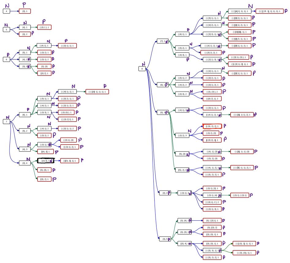
Figure 4 (click to view enlarged)
Observing the tree graphs for the first five possible game boards doesn't demonstrate a clear strategy for one of the players to play. It appears that the optimal strategy and who has the optimal strategy depends on the initial number of micro-loops within the game board. One attempt at figuring out the dependences of the optimal strategy is labeling all the game states as either N-positions or P-positions. Since this is a normal, impartial, and combinatorial game, N-positions and P-positions can be found using the following three conditions: all terminal positions are P-positions; from every N-position, there is at least one move to a P-position, and from every P-position, every move is to an N-position (Ferguson 5). Figure 4 displays the first five tree graphs with labeled N-positions and P-positions. These tree graphs demonstrate that all of the initial game states, except for the one containing an initial micro-loop number of 6, are N-positions. An N-position is a game state such that the next player has the winning strategy. In this case, the next player is the first player since that individual performs the first move. The initial game state for the game board containing and initial micro-loop number of 6 is a P-position. Thus, the previous player, or the second player, has the winning strategy. These results reflect previous findings when analyzing the fairness of the game using tree graphs. As one looks closely at these tree graphs, there doesn't appear to be an obvious strategy for a player to win because at each game state, a completely different move is performed. It is possible that there is a pattern by induction as one increases the initial amount of micro-loops within the game board, such that finding the modulus of that amount with a certain number provides the information of whether the first or second player will win. However, this would not benefit the general strategy analysis and it would be a difficult task to find such a pattern, since it seems as if the complexity of the game increases exponentially as one adds another initial micro-loop to the board.
Another attempt in finding a strategy is to create an algorithm that simulates the game in order to better understand any possible structures of the game and exploit a winning strategy. In order to efficiently simulate the game board, it would be ideal to use the Python (2.7) data structure of lists. Lists have special characteristics that enable them to be ideal for the task of representing loops. For example, lists are mutable and they can be nested within each other, just like the loops of the game. The algorithm created for the game (viewable on the last page of this report), in this attempt, reflected the complexity of the game and seemed quite abstract. There were difficulties dealing with mutating deeply nested lists which was fixed by repeating a few sub-algorithms. Essentially, these sub-algorithms could be converted to procedures but the danger of variable substitution and bringing back values from nested procedures kept this suggestion from consideration. Thus, no strategic value was gained from creating the algorithm.
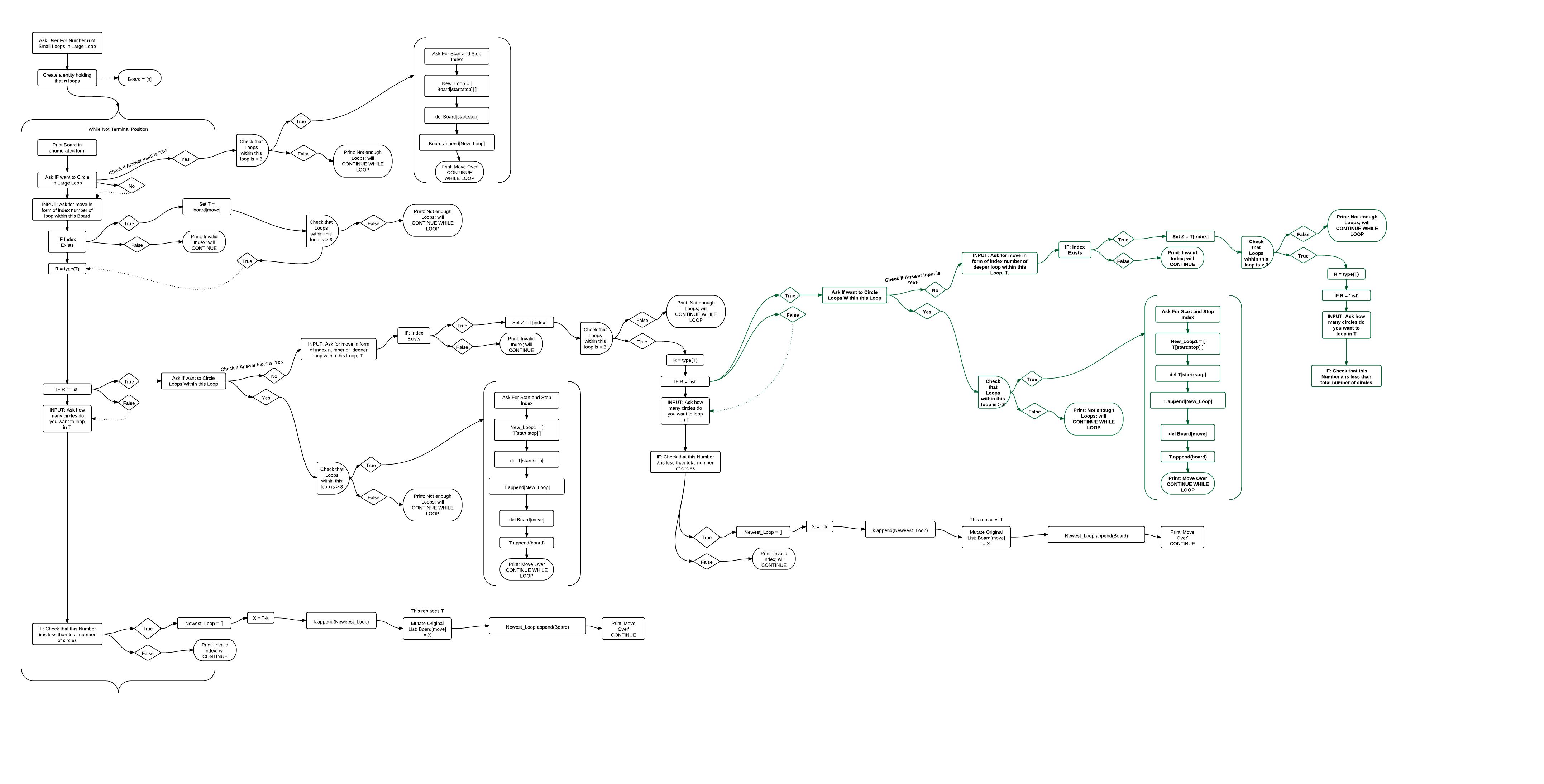
This is a flow chart of the algorithm created for the strategy. (click to view enlarged)
So far, the intricacy of the game seems to be an obstacle for finding the optimal game strategy. Perhaps, simplifying the rules of the game would provide more intuition of an optimal strategy. One possible way of narrowing the game down is to allow only three micro-loops to be fused into one macro-loop only if these micro-loops are found within a group of four or more micro-loops. Figure 5 demonstrates the first six possible tree graphs of this altered game. This altered version of Loop the Loop provides quicker insight to the complexity of the game, such as the ability to count macro-loops as micro-loops within certain perspectives. However, it doesn't provide insight to an optimal strategy of the original Loop the Loop. The tree graphs indicate that both versions are very different in complexity.
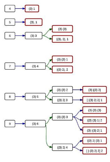
Figure 5 (click to view enlarged)
If you have any questions, feel free to email me.